Introduction to Android NDK

Introduction

To develop applications for Android OS, Google offers two development packages: SDK and NDK. There are many articles and books as well as good guidelines from Google about SDK. But even Google does not provide enough materials about NDK. Among all the existing books, I would like to single out only this one, “Cinar O. - Pro Android C++ with the NDK – 2012.” 

This article is intended for those with a lack of (or some) background in Android NDK who would like to strengthen their knowledge. I will pay attention to JNI. It seems to me that I have to start just from this interface. Also, at the end, we will review a short example with two functions of file writing and reading.

What is Android NDK?

Android NDK (Native Development Kit) is a set of tools that allows you to implement a part of your application using such languages as С/С++.

When to use the NDK?

Google recommends using NDK only in rare cases. Usually, these cases are the following:

• Necessity to increase performance (e.g. sorting of large data volumes);
• Use of a third-party library. For example, many applications are written in the С/С++ languages and it is necessary to use the existing material. Examples of such libraries are Ffmpeg, OpenCV;
• Programming on low level (for example, everything what goes beyond Dalvik).

What is JNI?

Java Native Interface is a standard mechanism for code execution under control of the Java Virtual Machine. The code is written in Assembler or С/С++ and assembled as dynamic libraries. It allows for the non-usage of the static binding. This provides an opportunity to call a С/С++ function from the program on Java and vice versa. 

JNI Advantages

The main competitive advantage of JNI compared to its analogues (Netscape Java Runtime Interface or Microsoft’s Raw Native Interface and COM/Java Interface) is that it was initially developed for ensuring binary compatibility, for compatibility of applications written for JNI, for any Java virtual machines on the concrete platform (while speaking about JNI, I do not mean the Dalvik machine as JNI was written by Oracle for JVM which is suitable for all Java Virtual Machines). That is the reason the compiled code on С/С++ will be executed regardless of platform. Earlier versions did not allow for the implementation of binary compatibility.   

Binary compatibility is a program compatibility type. It allows a program to work in different environments without changing its executable files.

Organization of JNI

Figure 1. – JNI – Interface pointer

The JNI table is organized like a table of virtual functions in С++. The VM can work with several such tables. For example, one will be for debugging, the other for usage. The JNI interface pointer is only valid in the current thread. This means that the pointer cannot move from one thread into another. However, native methods can be called from different threads.

Example:

jdouble Java_pkg_Cls_f__ILjava_lang_String_2 (JNIEnv *env, jobject obj, jint i, jstring s)
{
     const char *str = (*env)->GetStringUTFChars(env, s, 0); 
     (*env)->ReleaseStringUTFChars(env, s, str); 
     return 10;
}

• *env – an interface pointer;
• оbj – a reference to the object inside which the native method is declared;
• i and s – passed arguments;

Primitive types are copied between the VM and native code and objects are passed by the reference. The VM should trace all references that are passed to native code. GC cannot free all references passed to native code. But at the same time native code should inform the VM that it does not need references for passed objects.

Local and Global References

JNI defines three reference types: local, global and weak global references. Local ones are valid until the method is finished. All Java objects returned by JNI functions are local references. A programmer should hope that the VM would clean all local references. Local references are available only in the thread where they were created. However, if it is necessary they can be freed at once using DeleteLocalRef the JNI method of the interface:

jclass clazz;
clazz = (*env)->FindClass(env, "java/lang/String");
...
(*env)->DeleteLocalRef(env, clazz);

Global references remain valid until they are explicitly freed. To create a global reference you have to call a NewGlobalRef method. If the global reference is unnecessary, then it can be deleted by the DeleteGlobalRef method:

jclass localClazz;
jclass globalClazz;
...
localClazz = (*env)->FindClass(env, "java/lang/String");
globalClazz = (*env)->NewGlobalRef(env, localClazz);
...
(*env)->DeleteLocalRef(env, localClazz);

Errors

JNI does not check for errors such as NullPointerException, IllegalArgumentException. Reasons:

• decrease in performance;
• in the most C libraries functions, it is very difficult to be protected from errors.

JNI allows for the usage of Java Exception. Most JNI functions return an error code but not Exception itself. Therefore, it is necessary to handle the code itself and throw Exception to Java. In JNI, the error code of the called functions should be checked and after that ExceptionOccurred() should be called to return an error object: 

jthrowable ExceptionOccurred(JNIEnv *env);

For example, some JNI functions of access to arrays don’t return errors. But they can call the exception ArrayIndexOutOfBoundsException or ArrayStoreException.

JNI Primitive Types

In JNI exists its own primitive and reference types of data.
Table 1. Primitive types.

Java Type	Native Type	Description
boolean	jboolean	unsigned 8 bits
byte	jbyte	signed 8 bits
char	jchar	unsigned 16 bits
short	jshort	signed 16 bits
int	jint	signed 32 bits
long	jlong	signed 64 bits
float	jfloat	32 bits
double	jdouble	64 bits
void	void	N/A

JNI Reference Types 

Figure. 2 – JNI reference types

Modified UTF-8

The JNI uses modified UTF-8 strings to represent different string types. Java uses UTF-16. UTF-8 is mainly used in C because it encodes \u0000 as 0xc0, instead of the usual 0x00. Modified strings are encoded so that character sequences that contain only non-null ASCII characters can be represented using only one byte.  

JNI Functions: 

The JNI interface includes not only its own dataset but also its own functions. It will take a lot of time to review the dataset and functions since there are plenty of them. You can find out more information from the official documentation: http://docs.oracle.com/javase/6/docs/technotes/guides/jni/spec/functions.html

Sample of using JNI functions 

Below you will find a short example in order to make sure that you have correctly understood the material covered:

#include <jni.h>
    ...
JavaVM *jvm;
JNIEnv *env;
JavaVMInitArgs vm_args;
JavaVMOption* options = new JavaVMOption[1];
options[0].optionString = "-Djava.class.path=/usr/lib/java";
vm_args.version = JNI_VERSION_1_6;
vm_args.nOptions = 1;
vm_args.options = options;
vm_args.ignoreUnrecognized = false;
JNI_CreateJavaVM(&jvm, &env, &vm_args);
delete options;
jclass cls = env->FindClass("Main");
jmethodID mid = env->GetStaticMethodID(cls, "test", "(I)V");
env->CallStaticVoidMethod(cls, mid, 100);
jvm->DestroyJavaVM();

Let’s analyze by string:

• JavaVM – provides an interface for calling functions which allows for the creation and removal of JavaVM;
• JNIEnv – ensures most of the JNI functions;
• JavaVMInitArgs – arguments for JavaVM;
• JavaVMOption – options for JavaVM;

The JNI_CreateJavaVM() method initializes JavaVM and returns a pointer to the JNI interface pointer.
JNI_DestroyJavaVM() method loads the created JavaVM. 

Threads 

The kernel manages all the threads running on Linux; still they can be attached to the JavaVM via functions AttachCurrentThread and AttachCurrentThreadAsDaemon. If the thread is not attached, it has no access to JNIEnv. Android doesn’t stop the threads created from JNI, even if the GC is running.  The thread remains attached until it calls for the DetachCurrentThread method to detach itself from JavaVM.

First Steps

The structure of your project should look as is shown in Figure 3:

Figure. 3 – Project Structure

As Figure 3 shows, all the native code is stored to a jni folder. After a project build, the Libs folder should be separated into four subfolders. It means, one separate native library for each processor architecture. The quantity of libraries depends on the quantity of architectures selected. 

To create a native project, create a mere Android project and follow the steps: 

• Create a jni folder –  project sources root folder with native code sources;
• Create an Android.mk to build a project;
• Create an Application.mk to store compilation details. It is not required but is recommended as it allows for flexible compilation setting;
• Create an ndk-build file that will launch the compilation process (also not required).

Android.mk

As it was mentioned before, Android.mk is a makefile for native project compilation. Android.mk is used to group your code into modules. Under modules I mean statistic libraries, copied into the libs folder of your project, shared libraries and standalone executable.

Example of minimal configuration:

LOCAL_PATH := $(call my-dir)
include $(CLEAR_VARS)
LOCAL_MODULE    := NDKBegining
LOCAL_SRC_FILES := ndkBegining.c
include $(BUILD_SHARED_LIBRARY)

Let’s take a detailed look at:

• LOCAL_PATH := $(call my-dir) – function call my-dir is used to return the path of the folder the file is called in;
• include $(CLEAR_VARS) - cleans all the variables except LOCAL_PATH. It’s necessary to take into account as all the files are compiled in a single GNU Make context where all the variables are global;
• LOCAL_MODULE – The name of the output module. In the above-mentioned example, the output module name is set as NDKBegining, but after the build, libNDKBeginin libraries are created in the libs folder. Android adds a lib prefix to the name, but in java code you should indicate the library name without a prefix (that is, the name should be the same as in makefiles);
• LOCAL_SRC_FILES – listing source files to be built;
• include $(BUILD_SHARED_LIBRARY) points type of the output module.

One may set custom variables in Android.mk; however they must stick to the following syntax: LOCAL_, PRIVATE_, NDK_, APP_, my-dir. Google recommends naming custom examples as MY_. For example:

MY_SOURCE := NDKBegining.c

To call a variable $(MY_SOURCE)
Variable can also be concatenated, for example:

LOCAL_SRC_FILES += $(MY_SOURCE)

Application.mk

This makefile defines several variables that make compilation more flexible:

• APP_OPTIM – optional variable which is set either to release or debug. This variable is used for optimization when building an application's modules. You may manage release as debug; however debug gives more information for settings;
• APP_BUILD_SCRI defines an alternate path to Android.mk;
• APP_ABI – is probably one of the most essential variables. It specifies target processor architecture to compile the modules. By default, APP_ABI is set to 'armeabi', which corresponds to ARMv5TE architecture. For example, to support ARMv7, armeabi-v7a should be used; for IA-32– x86, for MIPS – mips, whereas for multiple architectures support, you should set APP_ABI := armeabi armeabi-v7a x86 mips. With NDK revision 7 and higher, you can simply set APP_ABI := all  rather than enumerating all the architectures. 
• APP_PLATFORM – names a target platform;
• APP_STL Android provides a very minimal libstdc++ runtime library so a developer is limited in using C++ functionality. However, APP_STL variable enables support for the extended functionality; 
• NDK_TOOLCHAIN_VERSION – enables the selection of a GCC compiler version (which, by default, is set to 4.6)

NDK-BUILDS

ndk-build is a wrapper around GNU Make.

After the 4th revision, flags were implemented for ndk-build: 

• clean – cleans all the generated binary files;
• NDK_DEBUG=1 – generates a debuggable code;
• NDK_LOG=1 – displays log messages (is used for debugging);
• NDK_HOST_32BIT=1 – Android supports 64-bit utilities version (for example, NDK_PATH\toolchains\mipsel-linux-android-4.8\prebuilt\windows-x86_64, etc. );
• NDK_APPLICATION_MK=<file> – indicates path to Application.mk.

In NDK revision 5, the NDK_DEBUG flag was introduced. When it is set to “1” the debug version will be built. If the flag is not set, the ndk-build by default will verify whether the attribute android:debuggable="true" is set in AndroidManifest.xml. If you are using NDK above revision 8, Google does not recommend using attribute android:debuggable in AndroidManifest.xml. (As you are using “ant debug” or building the debug version by the means of and ADT plug-in, the NDK_DEBUG=1 flag will be added automatically). 

By default, support of a 64-bit utilities version is set; however, you can force the use of a 32-bit toolchain by using NDK_HOST_32BIT=1. Still, Google recommends using 64-bit utilities to improve performance of the large programs. 

How to build a project?

It used to be a painful process. You would install CDT plug-in and download cygwin or mingw compiler; download Android NDK; configure all this stuff in Eclipse settings; and finally, it won’t work. The first time I started working with Android NDK, it took me three days to configure all these things. The problem was in Cygwin: the permission 777 should have been set to the project folder. 

Now it’s much easier. Just follow this link http://developer.android.com/sdk/index.html and download the ADT Bundle, which provides everything you need to start compiling. 

Invoke the native methods from Java code

To call native code from Java, first of all you need to define native methods in Java class. For example: 

native String nativeGetStringFromFile(String path) throws IOException;
native void nativeWriteByteArrayToFile(String path, byte[] b) throws IOException;

You should put the reserved word “native” before the method. In such a way, the compiler knows that this is an entry point in the JNI. These methods should be implemented in C/C++ files. Google also recommends starting naming methods with nativeX, where X stands for the method’s actual name.  Still, before implementing these methods manually you should generate a header file. You can perform this action either manually or using a JDK javah utility. Let’s take it a step further and not run it from the console, but rather by the standard Eclipse means.

• Go to Eclipse and select Run-External Tools-External Tools Configuration;
• Create new configuration;
• Indicate the path to javah.exe from jdk in Location field (for example, C:\Program Files (x86)\Java\jdk1.6.0_35\bin\javah.exe);
• Indicate the path to the directory bin/classes (for example, «${workspace_loc:/NDKBegin/bin/classes}») in the working directory;
• Arguments should be populated with the following argument: “-jni ${java_type_name}” (with no inverted commas).

Now we can run it. Your header files will be stored in the bin/classes directory. 

As a next step, copy these files into the jni directory of the native project. Next, open the project’s context menu and select Android Tools – Add Native Library. This allows us to use jni.h functions. Later on you can create a cpp file (sometimes Eclipse creates it by default) and write methods bodies that have been defined in the header file.   

You won’t find here a sample of code, as I haven’t inserted it on purpose, for the sake of the article’s length and readability.  Please follow the link on GitHub if you need an example https://github.com/viacheslavtitov/NDKBegining

RRD and rrdtool, sar graphs using pyrrd

Rather beautiful and ostensive graphs, don't you think? :)

This was always my weakness — representing dull statistic numbers in obvious and informative form — and if you share it with me, today I will tell you about RRD and rrdtool - rather easy and customizable tools for storing statistic data and building graphs from stored information.

Basic theory - explanation by simple example

RRD (round-robin database) — is a database, which has costant size and constant quantity of records. All the records in RRD are stored cyclically. What does it mean?

Let's imagine that you want to store results of pinging host for last 24 hours, in miliseconds. Ping command is executed every 5 minutes, so the result will be written to database every 300 seconds. A little math:

(60*60*24) / 300 = 288

This means that our database will have constant quantity of 288 rows. After the first 288 records old records, starting from the first one, will be deleted, and new ones will be added to the end of database.

Now let's complicate our task a bit. We want to save ping results for the last month. Ping command is executed every 5 minutes (300 seconds), but we don't need such an accuracy for month's statistics, so we can setup our database to insert records every hour. This means, that our database will store in cache 12 values for the last 60 minutes and will add to database one of the values: AVERAGE, MINIMUM, MAXIMUM or LAST, this depends on configuration of database.

(60*60*24*31) / 300 / 12 = 744

So, we will need 744 rows to store ping statistics per month.

Explanation in RRD "language"

First of all - rrd database must have at least one Data Source (DS). This is the structure of DS:

DS:variable_name:DST:heartbeat:min:max

• variable_name — a name for variable that will be used to access data from database.
• DST (Data Source Type) can be one of the next variants
  1. COUNTER — saves the rate of change; best to save data that allways increases (amount of traffic, and so on);
  2. DERIVE — same as COUNTER, but allows negative rates;
  3. ABSOLUTE - saves the rate of change, but it assumes that the previous value is set to 0; it is good if we want to count events after the last data input;
  4. GAUGE — saves the values itself, not the rate; best for storing monitoring data — CPU load, memory usage, ping miliseconds, and so on.
• heartbeat — time between two data inputs, in seconds.
• min and max — minimal and maximal values for input data.

So, accordingly to our example, DS will look this way:

DS:ping_ms:GAUGE:300:0:100000

Variable name is 'ping_ms', Data Source Type is GAUGE, and heartbeat is set to 300 seconds, because we execute ping command every 300 seconds. Minimal value is 0, and maximun value is set to 100000.

Also RRD must include at least one Round-robin Archive (RRA). RRA's structure:

RRA:CF:xff:step:rows

Input data comes to database through DS every 300 seconds. step parameter sets how many values of input data should be in cache before a Consolidation Function (CF) could be applied to them. rows parameter sets how many values will contain this RRA.

Let's get back to our example.

Our RRD will include 2 RRA — for last 24 hours and last 31 day. So, here is the first RRA:

RRA:AVERAGE:0.5:1:288

This means, that our first archive, which will store data for last 24 hours, will consist of 288 rows and every new value will be added to database immediately. CF can be ignored in this case, because no values will be placed in cache.

Second RRA:

RRA:AVERAGE:0.5:12:744

This archive will store info for last 31 day and will contain 744 rows. Every new value will be placed in cache. Then amount of values in cache reaches 12, CF will be applied to them. In our case CF is AVERAGE, which means that arithmetic average of values in cache will be inserted in database. Other possible CFs are:

• MINIMUM — minimum value in cache;
• MAXIMUM — maximum value in cache;
• LAST — last value in cache.

In addition, if we are talking about our example, the host we are pinging can be unreachable for some time. In this case the input data will be a special RRD type called UNKNOWN. xff — is a float parameter, from 0 to 1, which sets the maximum percentage of UNKNOWN values in cache, at which the applying of CF is allowed. For our second RRA xff is set to 0.5, which means that CF will be applied only if amount of UNKNOWN values in cache is less or equal 6. xff for first RRA can be ignored.

Drawing techniques

After we have updated our RRD with some data we can easily create graphs based on data, fetched from RRD. All the practical steps are described in section below, but there are several points that you have to understand before we can create graphs:

1. Time period, that will be represented in graph, must be defined;
2. We must define default variable, which will be the source of data from our RRD database. In our case it is all values of ping_ms variable in RRA archive, which will be chosen automatically accordingly to a defined period of time. Here is the syntax for default variable:
   DEF:<default_variable_name>=<rrd_database_file>:<name_of_variable_in_rrd>:<consolidation_function>
   For example:
   DEF:ping_host=ping.rrd:ping_ms:AVERAGE
3. We can add more variables, based on default variable, and apply some math to them. All the additional calculations must be written as Reverse Polish Notation (RPN). There are two types of additional variables, that we can create:
   • VDEF: consolidation function will be applied to all values in RRA. It's syntax:
     VDEF:<variable_name>=<default_variable_name>,<condolidation_function>
     For example:
     VDEF:ping_average=ping_host,AVERAGE
   • CDEF: some calculation will be applied to all values in RRA. The calculation must be written as RPN expression. CDEF's syntax:
     CDEF:<variable_name>=<rpn_expression>
     For example - if ping_host is greater then ping_average , the value will be assigned to ping_over_average:
     CDEF:ping_over_average=ping_host,ping_average,GT,ping_host,0,IF
4. Every defined variable will be shown on a graph as a graphical element. There are 5 types of graphical elements: AREA, LINE1, LINE2, LINE3(number stands for width) and STACK. Please see the example below to understand how the variables must be connected with graphical elements.

Creating and updating database. Simple graph

Now, after some theory, let's try some practice. The main tool for working with RRD database is command-line utility rrdtool. There are modules for different languages(Perl, Python), but on closer inspection it becomes apparent that they are wrappers around rrdtool, so rrdtool is a must dependency for any RRD-module.

Let's create RRD database file, using Data Source and Round-Robin Archives from the example above. As I've already mentioned - one additional parameter is needed for creating RRD - initial start time, in unix timestamp format:

$ rrdtool create ping.rrd \
  --start 1386350100 \
  DS:ping_ms:GAUGE:300:0:100000 \
  RRA:AVERAGE:0.5:1:288 \
  RRA:AVERAGE:0.5:12:744

Several cheks, for peace of mind =):

$ file ping.rrd
  ping.rrd: RRDTool DB version 0003
$ rrdtool info ping.rrd
  filename = "ping.rrd"
  rrd_version = "0003"
  step = 300
  last_update = 1386350100
  ds[ping_ms].type = "GAUGE"
  ds[ping_ms].minimal_heartbeat = 300
  ds[ping_ms].min = 0.0000000000e+00
  ds[ping_ms].max = 1.0000000000e+05
  ds[ping_ms].last_ds = "UNKN"
  ds[ping_ms].value = 0.0000000000e+00
  ds[ping_ms].unknown_sec = 200
  rra[0].cf = "AVERAGE"
  rra[0].rows = 288
  rra[0].pdp_per_row = 1
  rra[0].xff = 5.0000000000e-01
  rra[0].cdp_prep[0].value = NaN
  rra[0].cdp_prep[0].unknown_datapoints = 0
  rra[1].cf = "AVERAGE"
  rra[1].rows = 744
  rra[1].pdp_per_row = 12
  rra[1].xff = 5.0000000000e-01
  rra[1].cdp_prep[0].value = NaN
  rra[1].cdp_prep[0].unknown_datapoints = 2

Now lets put some fake data in our RRD. $RANDOM - is a built-in bash variable(also available in ksh): each reference of this variable generates random integer number from 0 to 32767:

$ start_time="1386350100"
$ heartbeat="300"
$ for i in {1..20} \
  do \
  shift_time=$((heartbeat*i)) \
  input_time=$((start_time+shift_time)) \
  rrdtool update ping.rrd $input_time:$RANDOM \
  done

And fetch data from database, to be sure that data has arrived from Data Source:

$ last_shift=$((300*10))
$ rrdtool fetch ping.rrd AVERAGE \
  --start $start_time --end $((start_time+last_shift))
                        ping_ms

  1386350400: 1.2571000000e+04
  1386350700: 1.7505000000e+04
  1386351000: 5.7370000000e+03
  1386351300: 1.9321000000e+04
  1386351600: 6.6680000000e+03
  1386351900: 2.8170000000e+04
  1386352200: 3.1665000000e+04
  1386352500: 1.0403000000e+04
  1386352800: 3.8130000000e+03
  1386353100: 5.5630000000e+03
  1386353400: 5.3420000000e+03

Now the most interesting part - let's build graph from the values in RRD:

$ last_shift=$((300*20))
$ rrdtool graph ping_graph.png \ 
  --start $start_time --end $((start_time+last_shift)) \
  DEF:ping_host=ping.rrd:ping_ms:AVERAGE \
  VDEF:ping_average=ping_host,AVERAGE \
  CDEF:ping_over_average=ping_host,ping_average,GT,ping_host,0,IF \
  CDEF:ping_below_average=ping_host,ping_average,LT,ping_host,0,IF \
  AREA:ping_over_average#FF0000:"ping over average" \
  AREA:ping_below_average#00FF00:"ping below average" \
  LINE1:ping_host#222222 \ 
  LINE2:ping_average#FFFF00:"average time of ping"
  481x168
$ file ping_graph.png
  ping_graph.png: PNG image data, 481 x 154, 8-bit/color RGBA, non-interlaced

To make things clear:

• output file for graph is image in PNG format;
• time period is creation time of RRD database + last_shift, which is egual to 300s * 20;
• default variable - is ping_ms for RRA archive, which suits the best for defined time period;
• VDEF variable, ping_average, is constant - it is the arithmetic average of all ping_ms values in RRA archive;
• first CDEF variable is ping_over_average - all the values which are greater then ping_average;
• second CDEF variable is ping_below_average - all the values which are less then ping_average;
• first graphical element: area, red colour - all the ping_over_average values, legend for graph is "ping over average";
• second graphical element: area, green colour - all the ping_below_average values, legend for graph is "ping below average";
• third graphical element: line, 1px width, dark grey colour - all the values of default variable;
• fourth graphical element: line, 2px width, yellow colour - horizontal line with constant value of ping_average, legend is "average time of ping".

And the graph itself:

Easy, isn't it?

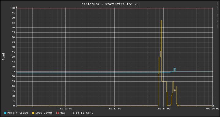
Complicated example — sar statistics, pyrrd

sar

sar — is a Unix tool for storing system activity reports. By default sar scripts, which gather information about system (CPU load, memory usage, i/o activity, etc), are launched via cron every 5 minutes and store statistic data in binary files. Here is an example output from sar file for the 17th day of current month, CPU load:

# sar -f /var/log/sa/sa17
...
12:00:01 AM       CPU     %user     %nice
12:05:01 AM       all      0.24      0.00
12:10:01 AM       all      0.25      0.00
12:15:01 AM       all      0.25      0.00 ...
...

And memory usage:

# sar -f /var/log/sa/sa17 -r
...
12:00:01 AM kbmemfree kbmemused  %memused kbbuffers
12:05:01 AM  11485772   4945420     30.10    325736
12:10:01 AM  11484664   4946528     30.10    325736
12:15:01 AM  11485508   4945684     30.10    325736 ...
...

Output of sar utility is just perfect to to be used as a source for RRD.

If you are using CentOS or RHEL, sar can be installed via yum; it is a part of sysstat package:

 # yum install sysstat

Post-installation scripts will also register jobs in cron, so you will need at least 1 hour after installation to get some reasonable output for RRD.

Setup python virtual environment

virtualenv is a tool, which creates isolated working copy of Python installation. You can work in virtual environments, install additional modules without affecting other Python installations. First of all we need to install python2.6, virtualenv and pip (a manager, which gives access to repository with python modules).

# yum install python26 python26-virtualenv python-pip

After installation we need to create virtual environment itself:

$ virtualenv-2.6 rrd_test
New python executable in rrd_test/bin/python2.6
Also creating executable in rrd_test/bin/python
Installing setuptools............done.

Now, let's activate new virtual environment:

$ . ./rrd_test/bin/activate
(rrd_test)$

Let's check the paths:

(rrd_test)$ which python2.6
~/temp/rrd_test/bin/python2.6
(rrd_test)$ which pip
~/temp/rrd_test/bin/pip

Everything seems fine, so the next step is to install pyrrd library using pip:

(rrd_test)$ pip install pyrrd
Downloading/unpacking pyrrd
  Downloading PyRRD-0.1.0.tar.gz (454Kb): 454Kb downloaded
...
Successfully installed pyrrd
Cleaning up...

Python script

I've decided that the best explanation of source code are profuse comments. Below you can see python script, which parses sar output, creates RRD databases, updates them with values from sar output, and draws graph for certain day of month.

I've called it sa2rrd.py. Please save it somewhere in virtual Python environment. Usage example:

(rrd_test)$ python2.6 sa2rrd.py --day <number_of_day>

Output PNG file will be in the directory with script and will look similar to this one:

Script's content can be found on pastebin.

Further investigation

If you are interested in the subject of the article - here are several points which may be worth attention:

• rrdcached - daemon, which caches input data. For highload systems;
• RRD-Simple - Perl module to manage RRD databases;
• modifying and customizing graphs accordingly to your needs; please see the documentation;
• RPN - theory, examples;
• more monitoring in Unix-like systems: additional sar parameters, ps, top(htop), iostat, lsof, vmstat, mpstat, netstat, socklist, tcpdump, nmap, ettercap, nagios(by the way - nagios is very friendly to RRD) and many others.

JSP Tag Library with Scala (taglib resurrection userguide)

Introduction

“What is dead may never die!”

―  George R. R. Martin, A Song of Ice and Fire

One can argue over what is dead and what is not for a long time. You can argue over anything, the main question is: is it worth doing that when you need to act? Necromancy has always been condemned, and that is actually right. But the cases are different. What would you do when you need the ‘dead’ to go?

JSTL overview

JSP Tag Library is a means of encapsulation of certain actions, which can be applied in Java Server Pages. Also, it should be mentioned that this is an effective means of code reusability, because the created tags can be used multiple times. And those are the things that may be very useful for Java developers working on the web.

It is worth noting that the library of custom tags is not quite a specific thing, but a logical supplement to JSP Standard Tag Library (although it may be vice versa). In fact, it would be strange to call something standard if there was not something non-standard. By the way, somehow it happened that when I heard about TagLib, I was not familiar with JSTL and immediately thought: "Aha, dear foreach, now I'll implement you once and for all," but it turned out that it had been already done before me (I cannot say I was very upset). That is why, not to reinvent the wheel, TagLib should be considered from the JSTL view.

To put it mildly, JSTL is an ancient technology, it appeared as early as in Java 1.4, so, if you are interested in details, the manuscripts documentation is always at your disposal. In turn, I will just give a quick overview of the things I’ve found interesting.

Thus, the standard tag library consists of several groups separated by functionality that is implemented by their components.

Core Tags

This group contains expression tags, remove tags (removing scoped variables), conditional tags, the already mentioned forEach, the redirect tag and some more tags the information about which you can find out by yourself.

Formatting tags

This group contains tags used for formatting and output of date, time and text, as well as tags dealing with localization from resources, such as the timeZone tag.

SQL tags

Hmm, don’t even know what to add. In general, the name of this group and <query>, <update> and <transaction> tags should speak for themselves.

XML tags

Pretty much the same as Core tags, but for XML. Except perhaps for the parse tag used to parse XML data from attribute or from tag body.

JSTL functions

These are not exactly tags. Or rather, these are not tags at all. This is just a set of functions used to work with string data. I think that you are familiar with such things as: contains, substring, trim ... Well, I told you.

Creating custom tag library

Generally speaking, to create your own tag library you don’t have to do much. Namely, you have to do two things:

1. Create a .tld file, which is essentially a XML document and describes the structure of your TagLib
2. Create a handler class that will describe the internal structure of the tag

This is in general. Now let’s consider in more detail what you need to do to come from nothing to the simplest, but working tag.

Tag Library Descriptor

A TLD should be created in the /META-INF/ directory or in any other of its subdirectories. The one, who has read the documentation or tutorial on TagLib, may note that the location of a TLD file depends on how we're going to pack the project, and will be absolutely right. The method described by me is suitable for the case when the project is packed in a JAR, but if you choose the way of WAR, then the TLD must be in the /WEB-INF/ directory. My choice is explained by the fact that, in my opinion, it’s much more logical, when the library is in a JAR file and can be connected to any project, rather than created and used only in one.

Here is a simple example of a TLD:

<?xml version="1.0" encoding="UTF-8" ?>

<taglib

     xmlns="http://java.sun.com/xml/ns/javaee"

     xmlns:xsi="http://www.w3.org/2001/XMLSchema-instance"

     xsi:schemaLocation="http://java.sun.com/xml/ns/javaee

     http://java.sun.com/xml/ns/javaee/web-jsptaglibrary_2_1.xsd"

     version="2.1">

     <tlib-version>1.0</tlib-version>

     <short-name>scltg</short-name>

     <uri>http://taglib.test.eleks.com</uri>

     <tag>

          <name>smpl</name>

          <tag-class>com.eleks.test.taglib.SimpleHandler</tag-class>

          <body-content>empty</body-content>

     </tag>

</taglib>

Colored with dumpz.org

All that interests us here is the <uri> tag, the content of which will help us in declaring the library on the JSP and the <tag> tag, remarkable for its almost recursivity, and that it still describes something that we are striving for so hard. In <tag-class>, you should indicate the fully qualified name of the tag handler class.

It should be added that there is a way of describing tags by tag files, but for convenience, I’ve done what I’ve done. If anyone is interested, they can look for the alternative option by themselves.

Tag handler class

There you go. We’ve got around to it. Get ready, there will be a surprise right now.

package com.eleks.test.taglib

import java.io.IOException

import javax.servlet.jsp.tagext.SimpleTagSupport

import javax.servlet.jsp.JspException

class SimpleHandler extends SimpleTagSupport {

     @throws [IOException]

     @throws [JspException]

     override def doTag() {

          getJspContext().getOut()
               .write("Hello, I'm a simple Scala tag!");

     }

}

Colored with dumpz.org

Strange annotation, strange "override def"… Yep, it’s Scala. 

For those who are greatly worried, I’m showing the same handler code for Java:

public class SimpleHandler extends SimpleTagSupport {

     public void doTag() throws JspException, IOException {

          getJspContext().getOut()
               .write("Hello, I'm a simple Java tag!");

     }

}

Colored with dumpz.org

I inherited from SimpleTagSupport to facilitate my work. In fact, there is an array of possible outcomes, and as always you can view the documentation for details.

That's all, it seems. I will also say a few words about how it all works, so you know which way to go.

In order to combine Java and Scala, a separate Maven project was created, which, as I have said, was compiled in a jar file. You can google for tutorials, so I won’t go into details, not to increase the entropy. Ok, but as for Pom.xml ― only things concerning Scala:

<properties>

     <scala.version>2.10.2</scala.version>

</properties>

<repositories>

     <repository>

          <id>scala-tools.org</id>

          <name>Scala-Tools Maven2 Repository</name>

          <url>http://scala-tools.org/repo-releases</url>

     </repository>

</repositories>

<pluginRepositories>

     <pluginRepository>

          <id>scala-tools.org</id>

          <name>Scala-Tools Maven2 Repository</name>

          <url>http://scala-tools.org/repo-releases</url>

     </pluginRepository>

</pluginRepositories>

<dependencies>

     <dependency>

          <groupId>org.scala-lang</groupId>

          <artifactId>scala-library</artifactId>

          <version>${scala.version}</version>

     </dependency>

<dependencies>

<build>

     <sourceDirectory>src/main/scala</sourceDirectory>

     <testSourceDirectory>src/test/scala</testSourceDirectory>

     <plugins>

          <plugin>

               <groupId>org.scala-tools</groupId>

               <artifactId>maven-scala-plugin</artifactId>

               <executions>

                    <execution>

                         <phase>compile</phase>

                         <goals>

                              <goal>compile</goal>

                              <goal>testCompile</goal>

                         </goals>

                    </execution>

               </executions>

               <configuration>

                    <scalaVersion>${scala.version}</scalaVersion>

                    <args>

                         <arg>-target:jvm-1.5</arg>

                    </args>

               </configuration>

          </plugin>

     </plugins>

</build>

Colored with dumpz.org

To use the tag library I’ve created another Maven project, which stated the following in the pom.xml file:

<dependencies>

     <dependency>

          <groupId>com.eleks.test</groupId>

          <artifactId>taglib</artifactId>

          <version>0.0.1-SNAPSHOT</version>

          <scope>import</scope>

     </dependency>

</dependencies>

Colored with dumpz.org

Everything is easy.

Using on the JSP

So, here is an example of JSP using the library written by us:

<%@ page language="java" contentType="text/html; charset=ISO-8859-1"

pageEncoding="ISO-8859-1"%>

<%@ taglib uri="http://taglib.test.eleks.com" prefix="scltg" %>

<!DOCTYPE html PUBLIC "-//W3C//DTD HTML 4.01 Transitional//EN" "http://www.w3.org/TR/html4/loose.dtd">

<html>

     <head>

          <meta http-equiv="Content-Type" content="text/html; charset=ISO-8859-1">

          <title>Insert title here</title>

     </head>

     <body>

          <scltg:smpl/>

     </body>

</html>

Colored with dumpz.org

The important points are highlighted in grey. The first thing is what I’ve already mentioned — we declare our Taglib and specify a prefix, with which we will refer to tags. And the second thing is actually our tag call: prefix, colon, tag name. As you see, the tag has no body, it’s just because the following thing was declared in the TLD:

<body-content>empty</body-content>

That’s it.

Pre conclusion

It was really cool. Moreover, it works. How useful is it? Well, I don't know. It's useful the way something useful has to be. Neither more nor less.

Conclusion

“Many that live deserve death. And some that die deserve life. Can you give it to them? Then do not be too eager to deal out death in judgement.” 

― J.R.R. Tolkien, The Fellowship of the Ring

Technologies become obsolete. This is a fact. Those which had no time to become obsolete (and sometimes even just to grow into something really demanded) are forgotten, lost, discarded with outbursts : "But why do we need it, after all, there is the ‘technology name’.” The fashion in the world of IT is as whimsical as any other fashion. And there's nothing you can do about that. Not so long ago, PC came to replace huge computing machines with access through terminals, then they were followed by laptops, then by netbooks and tablets, then cloud technologies came. The circle has been closed?

Nevertheless, and even more, there is always a need to go back to something old. Why not do it using something new? Maybe I gave the answer for the case of the JSP Tag Library.

C++ Multithreading Support

C++11 Multithreading overview 

The C++11 standard provides multithreading support, including the following features: thread creation and management, mutexes, atomic objects, thread local storage and condition variables.

Thread creation and management is provided by the std::thread class which is defined in <thread>. The class works with regular functions, lambdas (functions written directly in your source code) or functors (classes with overloaded () operator).  Any number of parameters can be passed to the thread function.  To work with the thread you should create an instance of std::thread class and pass it the working function.  Let’s see the example:

#include <iostream>

#include <thread>

void testFunc()

{

       std::cout << "Hello from the thread!";

}

int main(int argc, char *argv [])

{

       std::thread my_thread(testFunc);

       my_thread.join();

       return 0;

} 

In this example a reference to the trivial function is being passed to the constructor of the thread class. After thread creation we call join() to ensure that it has finished executing before program exit. Technically you should check whether the thread is joinable by calling its joinable() method first. If you don’t want to wait for thread execution finish, you could call the detach() member function to separate thread execution from the thread object. After calling detach() this thread object is no longer joinable. Any number of arguments can be passed to a thread:

#include <iostream>

#include <thread>

void printEven(int printArray[], int size)

{

       for (int i = 0; i < size; ++i)

       {

             if (printArray[i] % 2 == 0)

                    std::cout << "Even number " << i << " is - " << printArray[i] << "\n";

       }

}

int main(int argc, char *argv [])

{

       const int SIZE = 7;

       int evenArray[SIZE] = { 0, 7, 8, 63, 81, 24, 369 };

       std::thread my_thread(printEven, evenArray, SIZE);

       if (my_thread.joinable())

             my_thread.join();

       return 0;

} 

If there is need to pass parameters by reference, they should be wrapped into std::ref or std::cref.
Each thread has its own id. std::thread class  has get_id() member function, which returns unique id for the thread. To get the id of the current thread std::this_thread::get_id() can be used.  Thread id's are stored in lightweight std::thread::id class.

Useful features 

There are several useful functions in this_thread namespace. yield() function is used to notify the thread scheduler that it should select another thread to run. Using yield() is rarely necessary. sleep_until() expects an instance of std::chrono::time_point class and stops execution till system clock reaches this point. sleep_for() expects an instance std::chrono:duration class and blocks thread execution for that certain time.

#include <iostream>

#include <thread>

const int MAX_DELAY = 10;

const int THREADS_NUMBER = 5;

void raceThread()

{

       int delay = rand() % MAX_DELAY;

       std::thread::id currentID = std::this_thread::get_id();

       std::cout << "Thread with id " << currentID << " started. Delay " << delay << " seconds\n";

       std::this_thread::sleep_for(std::chrono::seconds(delay));

       std::cout << "Finishing thread...\n";

}

int main(int argc, char *argv [])

{

      

       std::auto_ptr<std::thread> ThreadsArray[THREADS_NUMBER];

       for (int i = 0; i < THREADS_NUMBER; ++i)

       {

             ThreadsArray[i].reset(new std::thread(raceThread));

       }

       for (int i = 0; i < THREADS_NUMBER; ++i)

       {

             ThreadsArray[i]->join();

       }

       return 0;

} 
Please try to tun the listing above several times. As you can see the results are different every time. That's because each thread is printing information using stdout which is a shared resource. Because iutput is not synchronized between working threads, it's ownership could be easily "stolen" by another threads. The result of such unsynchronized access is undefined behaviour.

Mutex  is used to ensure that only one thread is working with the shared resource at the same time.  So lets talk a bit about how they are defined in C++ 11 standard. Class std::mutex is used for locking and unlocking shared resources.  Besides it, there are three different types of mutexes – std::timed_mutex – which difference from previous one only by having a possibility to lock some resource for a certain timeout, std::recursive_mutex – this kind of mutex allows a thread to recursivly lock a resource, by making additional calls to lock or try_lock The period of ownership ends when thread makes a matching number of calls to unlock. Attempting to recursively lock a regular mutex will cause a deadlock. std::recursive_timed_mutex– recursive mutex with timeout ability. Lets change previous example and make access to the shared resource managed as we want it to be.

#include <iostream>

#include <thread>

#include <mutex>

const int MAX_DELAY = 10;

const int THREADS_NUMBER = 5;

std::mutex g_mutex;

void raceThread()

{

       std::lock_guard<std::mutex> lock(g_mutex);

       int delay = rand() % 10;

       std::thread::id currerntId = std::this_thread::get_id();

       std::cout << "Thread with id " << currerntId << " started. Delay " << delay << " seconds\n";

       std::this_thread::sleep_for(std::chrono::seconds(delay));

       std::cout << "Finishing thread...\n";

} 

The main function is the same as in previous listing so we've just skipped it here.  

std::lock_guard  is a RAII-style wrapper for more convenient work with std::mutex, it locks on creation and releases the lock after destruction.Because of potential deadlock problems, it is strongly recommended to avoid locking several mutexes at one time. Unfortunately, sometimes more than one resource should be locked (e.g. you  are working with two distinct data items and each of them is protected by its own mutex). In that case std::unique_lock can be helpful. It has a similar functionality to lock_guard but besides that it has a mechanism for avoiding deadlocks in case each resource should be locked by different mutex. An additional argument is passed to its constructor which defines locking strategy. By passing std::defer_lock you can tell std::unique_lock not to acquire ownership of the mutex immediately, and then safely lock both resources by std::lock:

struct Account

{

    Account(float sum) : m_fValue(sum) {}

    float m_fValue;

    std::mutex m_Mutex;

};

void foo(Account &parentAcc, Account &childAcc, float amount)

{

    // don't actually take the locks yet

    std::unique_lock<std::mutex> lock1(childAcc.m_Mutex, std::defer_lock);

    std::unique_lock<std::mutex> lock2(parentAcc.m_Mutex, std::defer_lock);

    // lock both unique_locks without deadlock

    std::lock(lock1, lock2);

    childAcc.m_fValue -= amount;

    parentAcc.m_fValue += amount;

} 

Please keep in mind that behaviour of a program is undefined in case a mutex is destroyed while still owned by some thread. A thread owns the mutex since the time the mutex is successfully locked till  the call of unlock method. So you have to be sure that mutex is not locking anything before destroying it.

Condition variables are another synchronization primitive which is provided by the C++11 standard. It is always associated with mutexes and allows threads to communicate with each other. Also it allows multiple threads to wait for some certain condition to become true or for a specified timeout to expire .  To work with a condition variable thread must acquire a lock first and pass the lock to subsequent condition variable operations. This lock will be implicitly released when the thread starts to wait on the condition variable and when the thread is being awakened because of conditional variable wakeup. std::condition_variable can block threads until notification is received or timeout is expired and sometimes when spurious wakeup occurs.

Besides std::condition_variable, there is a std::condition_variable_any. Thing is std::condition_variable can  work only with std::unique_lock<std::mutex>, where std::condition_variable_any can work with any (possibly used-defined) type which meets the BasicLockable requirments. Besides that, functionality of both synchronization primitives is almost identical.

C++ threads vs. Boost threads

One of the most common used open-source libraries for C++ is Boost. This library also provides multithreading support, so let's compare C++11 threads with boost threads. C++11 threads are supported at core language level while boost threads are basically wrappers around platform-dependent thread implementations.

First thing which you may notice by now is that a C++ thread will not have its detach() method implicitly called when it is being destructed.  You have to manually call join() or detach() before destructing  a thread. If you don’t,  the program will call std::terminate() and it will abort your application.  In Boost there is no such problem because detach() is called automatically on thread destruction.  Boost threads support cancelation, but C++ standard threads don’t.
std::thread allows move-only types, such as  std::unique_ptr to be passed as arguments. Because of the use of boost::bind internally,  Boost requires copyable arguments.  To clear things up a little bit let's see an example:

void foo(std::unique_ptr<int>);

std::thread my_thread(foo, std::unique_ptr<int>(new int(228)));  

std::unique_ptr cannot be copied so this example won't work.  It works when using std::thread, but it won’t be working with boost::thread due to its semantics requiring copyable arguments. Migration from Boost threads to C++11 should not cause a lot of trouble. Of course, some of the Boost features are not supported in C++ standard yet. For example, there is no analogue of boost::shared_mutex, which allows multiple-reader and single-writer locking. It is planned to include such kind of mutex in future C++ standard (from C++14), but currently it is not implemented.Also using threads from the language standard gives few advantages comparing to usage of Boost threads.  No matter how convenient Boost is it’s still an additional library, which means you need to rely on Boost libraries during compilation and linkage. Sometimes these libraries need to be updated. When using C++ threads, which are already included into the standard you don’t  need to worry about such things.

How it works? 

We’ve seen the main features of the C++ threading model. Let’s try to use these features while solving some practical task. Producer-consumer is a well-known multithreading problem. It describes two threads working with a single queue. One of them produces something and puts it into queue and another is consuming and removes items from the queue. The main problem is to ensure that the producer won't try to add into the queue when it's full and consumer won't try to consume from the queue when it's empty.

Lets add some general variables which will be used by both threads.

bool g_isReady = false;

std::mutex g_Mutex;

std::condition_variable g_ConditionVar;

std::queue<int> g_MessagesQueue;

const int QUEUE_SIZE = 10;

const int SLEEP_TIME = 500; 

We declared a boolean flag to indicate ready status of queue, the global message queue to put data in it, and mutex for locking shared data while working with it. Also we a declare condition variable for communication between threads. To prevent hardcoding we declare constants for queue size and sleep time. Producer function will look like this:

void Producer()

{

       std::cout << "\\\\\ Producer is ready ///// \n";

      

       for( int i = 0; ; ++i )

       {

             std::this_thread::sleep_for(std::chrono::milliseconds(SLEEP_TIME));                   

             std::unique_lock<std::mutex> lock(g_Mutex);  

            

                            

             if ( g_MessagesQueue.size() < QUEUE_SIZE )

             {

                    std::cout << "Produced " << i << "\n";

                    g_MessagesQueue.push(i);    

             }

             else

             {

                    g_isReady = true; 

                    g_ConditionVar.notify_one();             

             }

       }

} 

Here we have a an infinite loop which pushes data to queue . On each iteration it has small delay and total number of queue elements is compared with queue size. If it less  than the maximum queue size data  is being pushed to the queue, otherwise the status flag is given the appropriate status and the condition variable is used to send notification to the consumer thread.  Lock is acquired when working with shared resources.     Now in the consumer function we have one more infinite loop. It uses the status flag which prevents it from spurious wakeups and waits for notification form the producer thread. After a notification has been received the consumer pops data from the queue and sets the status flag to false:

void Consumer()

{

       std::cout << "\\\\\ Consumer is ready ///// \n";

       while (true)

       {

             std::unique_lock<std::mutex> lock(g_Mutex);

             while (!g_isReady)                            

             {

                    g_ConditionVar.wait(lock);           

             }

             while (!g_MessagesQueue.empty())            

             {

                    std::cout << "Consumed -" << g_MessagesQueue.front() << "\n";

                    g_MessagesQueue.pop();

             }

             g_isReady = false;                           

       }

} 
In the main routine there are only threads creation and waiting them to finish.

int main(int argc, char *argv[])

{

       std::thread producer(Producer);

       std::thread consumer(Consumer);

       if (producer.joinable())

             producer.join();

       if (consumer.joinable())

             consumer.join();

}  
As you can see the C++11 standard presents some powerful features for multithreading support. These features are expected to be enhanced in the next C++ standards.